06: Logistic Regression

Classification

Where y is a discrete value
- Develop the logistic regression algorithm to determine what class a new input should fall into
Classification problems
- Email -> spam/not spam?
- Online transactions -> fraudulent?
- Tumor -> Malignant/benign
Variable in these problems is Y
- Y is either 0 or 1
  - 0 = negative class (absence of something)
  - 1 = positive class (presence of something)
Start with binary class problems
- Later look at multiclass classification problem, although this is just an extension of binary classification
How do we develop a classification algorithm?
- Tumour size vs malignancy (0 or 1)
- We could use linear regression
  - Then threshold the classifier output (i.e. anything over some value is yes, else no)
  - In our example below linear regression with thresholding seems to work

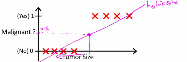
We can see above this does a reasonable job of stratifying the data points into one of two classes
- But what if we had a single Yes with a very small tumour
- This would lead to classifying all the existing yeses as nos
Another issues with linear regression
- We know Y is 0 or 1
- Hypothesis can give values larger than 1 or less than 0
So, logistic regression generates a value which is always between 0 and 1
- Logistic regression is a classification algorithm - don't be confused

Hypothesis representation

What function is used to represent our hypothesis in classification
We want our classifier to output values between 0 and 1
- When using linear regression we did h_θ(x) = (θ^T x)
- For classification hypothesis representation we do h_θ(x) = g((θ^T x))
  - Where we define g(z)
    - z is a real number
  - g(z) = 1/(1 + e^-z)
    - This is the sigmoid function, or the logistic function
  - If we combine these equations we can write out the hypothesis as
    $h_{θ} (x) = \frac{1}{1 + e^{- θ^{T} x}}$
```
import numpy as np

def g(z):   # the sigmoid function
    return 1 / (1 + np.exp(-z))

g(0)     # 0.5      - the crossing point
g(10)    # 0.99995  - asymptotes towards 1
g(-10)   # 0.00005  - asymptotes towards 0
```
    Crosses 0.5 at z = 0 and saturates in both directions — the shape drawn above.
What does the sigmoid function look like
Crosses 0.5 at the origin, then flattens out
- Asymptotes at 0 and 1

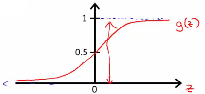
Given this we need to fit θ to our data

Interpreting hypothesis output

When our hypothesis (h_θ(x)) outputs a number, we treat that value as the estimated probability that y=1 on input x
- Example
  - If X is a feature vector with x₀ = 1 (as always) and x₁ = tumourSize
  - h_θ(x) = 0.7
    - Tells a patient they have a 70% chance of a tumor being malignant
- We can write this using the following notation
  - h_θ(x) = P(y=1|x ; θ)
- What does this mean?
  - Probability that y=1, given x, parameterized by θ
Since this is a binary classification task we know y = 0 or 1
- So the following must be true
  - P(y=1|x ; θ) + P(y=0|x ; θ) = 1
  - P(y=0|x ; θ) = 1 - P(y=1|x ; θ)

Decision boundary

Gives a better sense of what the hypothesis function is computing
Better understand of what the hypothesis function looks like
- One way of using the sigmoid function is;
  - When the probability of y being 1 is greater than 0.5 then we can predict y = 1
  - Else we predict y = 0
- When is it exactly that h_θ(x) is greater than 0.5?
  - Look at sigmoid function
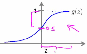
    - g(z) is greater than or equal to 0.5 when z is greater than or equal to 0
  - So if z is positive, g(z) is greater than 0.5
    - z = (θ^T x)
  - So when
    - θ^T x >= 0
  - Then h_θ >= 0.5
So what we've shown is that the hypothesis predicts y = 1 when θ^T x >= 0
- The corollary of that when θ^T x <= 0 then the hypothesis predicts y = 0
- Let's use this to better understand how the hypothesis makes its predictions

Decision boundary

h_θ(x) = g(θ₀ + θ₁x₁+ θ₂x₂)

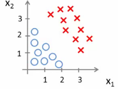
So, for example
- θ₀ = -3
- θ₁ = 1
- θ₂ = 1
So our parameter vector is a column vector with the above values
- So, θ^T is a row vector = [-3,1,1]
What does this mean?
- The z here becomes θ^T x
- We predict "y = 1" if
  - -3x₀ + 1x₁ + 1x₂ >= 0
  - -3 + x₁ + x₂ >= 0
We can also re-write this as
- If (x₁ + x₂ >= 3) then we predict y = 1
- If we plot
  - x₁ + x₂ = 3 we graphically plot our decision boundary

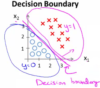
Means we have these two regions on the graph
- Blue = false
- Magenta = true
- Line = decision boundary
  - Concretely, the straight line is the set of points where h_θ(x) = 0.5 exactly
- The decision boundary is a property of the hypothesis
  - Means we can create the boundary with the hypothesis and parameters without any data
    - Later, we use the data to determine the parameter values
  - i.e. y = 1 if
    - 5 - x₁ > 0
    - 5 > x₁

Non-linear decision boundaries

Get logistic regression to fit a complex non-linear data set
- Like polynomial regression add higher order terms
- So say we have
  - h_θ(x) = g(θ₀ + θ₁x₁ + θ₂x₂ + θ₃x₁² + θ₄x₂²)
  - We take the transpose of the θ vector times the input vector
    - Say θ^T was [-1,0,0,1,1] then we say;
    - Predict that "y = 1" if
      - -1 + x₁² + x₂² >= 0
        or
      - x₁² + x₂² >= 1
    - If we plot x₁² + x₂² = 1
      - This gives us a circle with a radius of 1 around 0

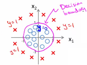
Mean we can build more complex decision boundaries by fitting complex parameters to this (relatively) simple hypothesis
More complex decision boundaries?
- By using higher order polynomial terms, we can get even more complex decision boundaries

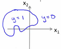
Cost function for logistic regression

Fit θ parameters
Define the optimization objective for the cost function we use to fit the parameters
- Training set of m training examples
  - Each example is an n+1 length column vector

Training set: {(x^{(1)}, y^{(1)}), (x^{(2)}, y^{(2)}), \dots, (x^{(m)}, y^{(m)})}

x \in [\begin{matrix} x_{0} \\ x_{1} \\ ⋮ \\ x_{n} \end{matrix}] x_{0} = 1, y \in {0, 1}

h_{θ} (x) = \frac{1}{1 + e^{- θ^{T} x}}

m examples, each a column vector of n+1 features.

This is the situation
- Set of m training examples
- Each example is a feature vector which is n+1 dimensional
- x₀ = 1
- y ∈ {0,1}
- Hypothesis is based on parameters (θ)
  - Given the training set how do we choose/fit θ?
Linear regression uses the following function to determine θ

J (θ) = \frac{1}{m} \sum_{i = 1}^{m} \frac{1}{2} {(h_{θ} (x^{(i)}) - y^{(i)})}^{2}

Instead of writing the squared error term, we can write
- If we define "cost()" as;
  - cost(h_θ(xⁱ), y) = 1/2(h_θ(xⁱ) - yⁱ)²
  - Which evaluates to the cost for an individual example using the same measure as used in linear regression
- We can redefine J(θ) as
  $J (θ) = \frac{1}{m} \sum_{i = 1}^{m} Cost (h_{θ} (x^{(i)}), y^{(i)})$
  - Which, appropriately, is the sum of all the individual costs over the training data (i.e. the same as linear regression)
To further simplify it we can get rid of the superscripts
- So
  $J (θ) = \frac{1}{m} \sum_{i = 1}^{m} Cost (h_{θ} (x), y)$
What does this actually mean?
- This is the cost you want the learning algorithm to pay if the outcome is h_θ(x) and the actual outcome is y
- If we use this function for logistic regression this is a non-convex function for parameter optimization
  - Could work....
What do we mean by non convex?
- We have some function - J(θ) - for determining the parameters
- Our hypothesis function has a non-linearity (sigmoid function of h_θ(x) )
  - This is a complicated non-linear function
- If you take h_θ(x) and plug it into the Cost() function, and then plug the Cost() function into J(θ) and plot J(θ) we find many local optimum -> non convex function
- Why is this a problem
  - Lots of local minima mean gradient descent may not find the global optimum - may get stuck in a local minimum
- We would like a convex function so if you run gradient descent you converge to a global minimum

A convex logistic regression cost function

To get around this we need a different, convex Cost() function which means we can apply gradient descent

Cost (h_{θ} (x), y) =

- \log (h_{θ} (x))

if y = 1

- \log (1 - h_{θ} (x))

if y = 0

This is our logistic regression cost function
- This is the penalty the algorithm pays
- Plot the function
Plot y = 1
- So h_θ(x) evaluates as -log(h_θ(x))

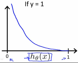
So when we're right, cost function is 0
- Else it slowly increases cost function as we become "more" wrong
- X axis is what we predict
- Y axis is the cost associated with that prediction
This cost functions has some interesting properties
- If y = 1 and h_θ(x) = 1
  - If hypothesis predicts exactly 1 and that's exactly correct then that corresponds to 0 (exactly, not nearly 0)
- As h_θ(x) goes to 0
  - Cost goes to infinity
  - This captures the intuition that if h_θ(x) = 0 (predict P (y=1|x; θ) = 0) but y = 1 this will penalize the learning algorithm with a massive cost
What about if y = 0
then cost is evaluated as -log(1- h_θ( x ))
- Just get inverse of the other function

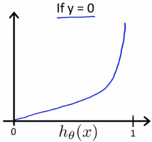
Now it goes to plus infinity as h_θ(x) goes to 1
With our particular cost functions J(θ) is going to be convex and avoid local minimum

Simplified cost function and gradient descent

Define a simpler way to write the cost function and apply gradient descent to the logistic regression
- By the end should be able to implement a fully functional logistic regression function
Logistic regression cost function is as follows

J (θ) = \frac{1}{m} \sum_{i = 1}^{m} Cost (h_{θ} (x^{(i)}), y^{(i)})

Cost (h_{θ} (x), y) =

- \log (h_{θ} (x))

if y = 1

- \log (1 - h_{θ} (x))

if y = 0

y is always 0 or 1.

This is the cost for a single example
- For binary classification problems y is always 0 or 1
  - Because of this, we can have a simpler way to write the cost function
    - Rather than writing cost function on two lines/two cases
    - Can compress them into one equation - more efficient
- Can write cost function is
  - cost(h_θ(x),y) = -ylog( h_θ(x) ) - (1-y)log( 1- h_θ(x) )
    - This equation is a more compact version of the two cases above
- We know that there are only two possible cases
  - y = 1
    - Then our equation simplifies to
      - -log(h_θ(x)) - (0)log(1 - h_θ(x))
        
        -log(h_θ(x))
        
        Which is what we had before when y = 1
  - y = 0
    - Then our equation simplifies to
      - -(0)log(h_θ(x)) - (1)log(1 - h_θ(x))
      - = -log(1- h_θ(x))
      - Which is what we had before when y = 0
  - Clever!
So, in summary, our cost function for the θ parameters can be defined as

J (θ) = - \frac{1}{m} [\sum_{i = 1}^{m} y^{(i)} \log h_{θ} (x^{(i)}) + (1 - y^{(i)}) \log (1 - h_{θ} (x^{(i)}))]

Because y is always 0 or 1, one of the two terms is always zero — so this single expression covers both cases.

def J(theta, X, y):
    h = g(X @ theta)
    return -(y * np.log(h) + (1 - y) * np.log(1 - h)).mean()

X = np.array([[1, 1], [1, 2], [1, 3], [1, 4]], dtype=float)
y = np.array([0, 0, 1, 1], dtype=float)

J(np.zeros(2), X, y)   # 0.6931 = log(2): with theta = 0 every h is 0.5

The compressed cost, vectorized. With θ = 0 the hypothesis says 0.5 for everything, and the cost is exactly log 2 per example.

Why do we choose this function when other cost functions exist?
- This cost function can be derived from statistics using the principle of maximum likelihood estimation (chapter 05)
  - Note this does mean there's an underlying probabilistic assumption - the labels, given x, are modelled as Bernoulli
- Also has the nice property that it's convex
To fit parameters θ:
- Find parameters θ which minimize J(θ)
- This means we have a set of parameters to use in our model for future predictions
Then, if we're given some new example with set of features x, we can take the θ which we generated, and output our prediction using
$h_{θ} (x) = \frac{1}{1 + e^{- θ^{T} x}}$
- This result is
  - p(y=1 | x ; θ)
    - Probability y = 1, given x, parameterized by θ

How to minimize the logistic regression cost function

Now we need to figure out how to minimize J(θ)
- Use gradient descent as before
- Repeatedly update each parameter using a learning rate

Repeat {

θ_{j} ≔ θ_{j} - α \sum_{i = 1}^{m} (h_{θ} (x^{(i)}) - y^{(i)}) x_{j}^{(i)}

}

simultaneously update all θ_j

theta = np.zeros(2)
for _ in range(20000):
    h = g(X @ theta)
    theta = theta - 0.5 * X.T @ (h - y) / len(y)

theta                  # [-25.6, 10.3]
-theta[0] / theta[1]   # 2.48 -> the decision boundary sits between x = 2 and x = 3
np.round(g(X @ theta), 3)   # [0., 0.007, 0.995, 1.]  - the fit

The same update as linear regression, but h is the sigmoid. The boundary lands at x ≈ 2.5 — between the last y = 0 example and the first y = 1.

If you had n features, you would have an n+1 column vector for θ
This equation is the same as the linear regression rule
- The only difference is that our definition for the hypothesis has changed
Previously, we spoke about how to monitor gradient descent to check it's working
- Can do the same thing here for logistic regression
When implementing logistic regression with gradient descent, we have to update all the θ values (θ₀ to θ_n) simultaneously
- Could use a for loop
- Better would be a vectorized implementation
Feature scaling for gradient descent for logistic regression also applies here

Advanced optimization

Previously we looked at gradient descent for minimizing the cost function
Here look at advanced concepts for minimizing the cost function for logistic regression
- Good for large machine learning problems (e.g. huge feature set)
What is gradient descent actually doing?
- We have some cost function J(θ), and we want to minimize it
- We need to write code which can take θ as input and compute the following
  - J(θ)
  - Partial derivative of J(θ) with respect to j (where j=0 to j = n)

J (θ)

\frac{\partial}{\partial θ_{j}} J (θ)

for j = 0, 1, …, n

Given code that can do these two things
- Gradient descent repeatedly does the following update

$Repeat {θ_{j} ≔ θ_{j} - α \frac{\partial}{\partial θ_{j}} J (θ)}$

So update each j in θ sequentially
So, we must;
- Supply code to compute J(θ) and the derivatives
- Then plug these values into gradient descent
Alternatively, instead of gradient descent to minimize the cost function we could use
- Conjugate gradient
- BFGS (Broyden-Fletcher-Goldfarb-Shanno)
- L-BFGS (Limited memory - BFGS)
These are more optimized algorithms which take that same input and minimize the cost function
These are very complicated algorithms
Some properties
- Advantages
  - No need to manually pick alpha (learning rate)
    - Have a clever inner loop (line search algorithm) which tries a bunch of alpha values and picks a good one
  - Often faster than gradient descent
    - Do more than just pick a good learning rate
  - Can be used successfully without understanding their complexity
- Disadvantages
  - Could make debugging more difficult
  - Should not be implemented yourself
  - Different libraries may use different implementations - may hit performance

Using advanced cost minimization algorithms

How to use algorithms
- Say we have the following example

θ = [\begin{matrix} θ_{1} \\ θ_{2} \end{matrix}]

J (θ) = {(θ_{1} - 5)}^{2} + {(θ_{2} - 5)}^{2}

\frac{\partial}{\partial θ_{1}} J (θ) = 2 (θ_{1} - 5)

\frac{\partial}{\partial θ_{2}} J (θ) = 2 (θ_{2} - 5)

from scipy.optimize import minimize

def cost_function(theta):
    jval = ((theta - 5) ** 2).sum()
    gradient = 2 * (theta - 5)
    return jval, gradient

res = minimize(cost_function, np.zeros(2), jac=True)
res.x   # [5., 5.]  - the minimum, exactly where the derivatives hit zero

The worked example above, run for real: minimize drives both parameters to 5 without us ever picking a learning rate.

Example above
- θ₁ and θ₂ (two parameters)
- Cost function here is J(θ) = (θ₁ - 5)² + ( θ₂ - 5)²
- The derivatives of the J(θ) with respect to either θ₁ and θ₂ turns out to be the 2(θ_i - 5)
First we need to define our cost function, which should have the following signature

def cost_function(theta):
    ...
    return jval, gradient

Input for the cost function is theta, which is a vector of the θ parameters
Two return values from cost_function are
- jval
  - How we compute the cost function θ (the underived cost function)
    - In this case = (θ₁ - 5)² + (θ₂ - 5)²
- gradient
  - 2 by 1 vector
  - 2 elements are the two partial derivative terms
  - i.e. this is an n-dimensional vector
    - Each indexed value gives the partial derivatives for the partial derivative of J(θ) with respect to θ_i
    - Where i is the index position in the gradient vector
With the cost function implemented, we can call the advanced algorithm using

from scipy.optimize import minimize

initial_theta = np.zeros(2)                  # initialize the theta values
res = minimize(cost_function, initial_theta, # run the algorithm
               jac=True, options={'maxiter': 100})
opt_theta, function_val = res.x, res.fun

Here
- options is a dictionary giving options for the algorithm
- minimize
  - SciPy's general-purpose cost function minimizer (scipy.optimize.minimize)
- cost_function is passed as an object - Python functions are first-class values, so no special syntax is needed
For this implementation
- jac=True tells minimize that cost_function returns the gradient along with the cost
How do we apply this to logistic regression?
- Here we have a vector

THETA = [\begin{matrix} θ_{0} \\ θ_{1} \\ ⋮ \\ θ_{n} \end{matrix}]

def cost_function(theta):

    jval = [code to compute  $J (θ)$ ];

    gradient[0] = [code to compute  $\frac{\partial}{\partial θ_{0}} J (θ)$ ];

    gradient[1] = [code to compute  $\frac{\partial}{\partial θ_{1}} J (θ)$ ];
     $⋮$ 
    gradient[n] = [code to compute  $\frac{\partial}{\partial θ_{n}} J (θ)$ ];

Here
- theta is a n+1 dimensional column vector
- NumPy indexes from 0, so gradient[0] is the θ₀ entry
Write a cost function which captures the cost function for logistic regression

Multiclass classification problems

Getting logistic regression for multiclass classification using one vs. all
Multiclass - more than yes or no (1 or 0)
- Classification with multiple classes for assignment

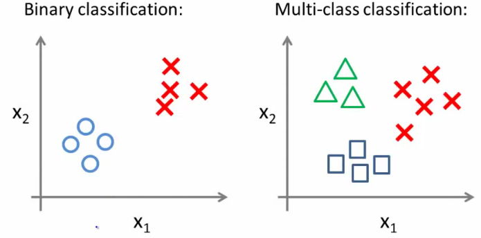
Given a dataset with three classes, how do we get a learning algorithm to work?
- Use one vs. all classification make binary classification work for multiclass classification
One vs. all classification
- Split the training set into three separate binary classification problems
  - i.e. create a new fake training set
    - Triangle (1) vs crosses and squares (0) h_θ¹(x)
      - P(y=1 | x₁; θ)
    - Crosses (1) vs triangle and square (0) h_θ²(x)
      - P(y=1 | x₂; θ)
    - Square (1) vs crosses and triangle (0) h_θ³(x)
      - P(y=1 | x₃; θ)

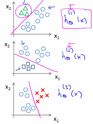
Overall
- Train a logistic regression classifier h_θ⁽ⁱ⁾(x) for each class i to predict the probability that y = i
- On a new input, x to make a prediction, pick the class i that maximizes the probability that h_θ⁽ⁱ⁾(x) = 1