14: Dimensionality Reduction (PCA)

Motivation 1: Data compression

Start talking about a second type of unsupervised learning problem - dimensionality reduction
- Why should we look at dimensionality reduction?

Compression

Speeds up algorithms
Reduces space used by data for them
What is dimensionality reduction?
- So you've collected many features - maybe more than you need
  - Can you "simplify" your data set in a rational and useful way?
- Example
  - Redundant data set - different units for same attribute
  - Reduce data to 1D (2D->1D)
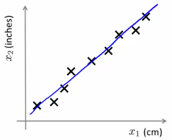
    - Example above isn't a perfect straight line because of round-off error
- Data redundancy can happen when different teams are working independently
  - Often generates redundant data (especially if you don't control data collection)
- Another example
  - Helicopter flying - do a survey of pilots (x1 = skill, x2 = pilot enjoyment)
    - These features may be highly correlated
    - This correlation can be combined into a single attribute called aptitude (for example)
What does dimensionality reduction mean?
- In our example we plot a line
- Take exact example and record position on that line
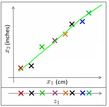
- So before x¹was a 2D feature vector (X and Y dimensions)
- Now we can represent x¹ as a 1D number (Z dimension)
So we approximate original examples
- Allows us to halve the amount of storage
- Gives lossy compression, but an acceptable loss (probably)
  - The loss above comes from the rounding error in the measurement, however
Another example 3D -> 2D
- So here's our data
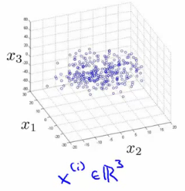
- Maybe all the data lies in one plane
  - This is sort of hard to explain in 2D graphics, but that plane may be aligned with one of the axes
    - Or may not...
    - Either way, the plane is a small, constant 3D space
  - In the diagram below, imagine all our data points are sitting "inside" the blue tray (has a dark blue exterior face and a light blue inside)
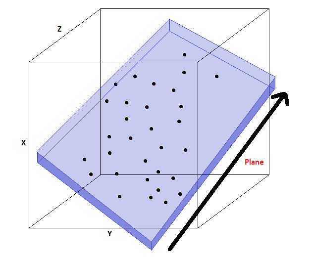
  - Because they're all in this relative shallow area, we can basically ignore one of the dimensions, so we draw two new lines (z1 and z2) along the x and y planes of the box, and plot the locations in that box
  - i.e. we lose the data in the z-dimension of our "shallow box" (NB "z-dimensions" here refers to the dimension relative to the box (i.e. its depth) and NOT the z dimension of the axis we've got drawn above) but because the box is shallow it's OK to lose this. Probably....
- Plot values along those projections
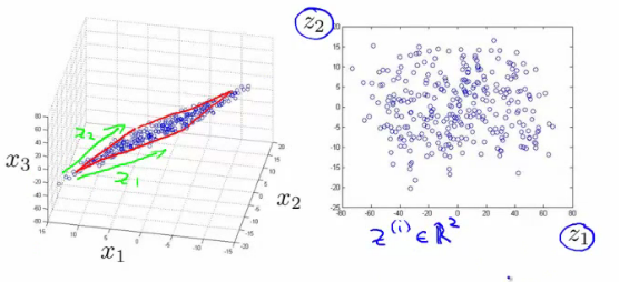
- So we've now reduced our 3D vector to a 2D vector
In reality we'd normally try and do 1000D -> 100D

Motivation 2: Visualization

It's hard to visualize highly dimensional data
- Dimensionality reduction can improve how we display information in a tractable manner for human consumption
- Why do we care?
  - Often helps to develop algorithms if we can understand our data better
  - Dimensionality reduction helps us do this, see data in a helpful way
  - Good for explaining something to someone if you can "show" it in the data

Example;

Collect a large data set about many facts of a country around the world

The first six of about fifty features per country. x₁ is GDP through to x₆, mean household income; the rest continue off the right.
Country	GDP (trillions of US$)	Per capita GDP (thousands of intl. $)	Human Development Index	Life expectancy	Poverty Index (Gini as percentage)	Mean household income (thousands of US$)	…
Canada	1.577	39.17	0.908	80.7	32.6	67.293	…
China	5.878	7.54	0.687	73	46.9	10.22	…
India	1.632	3.41	0.547	64.7	36.8	0.735	…
Russia	1.48	19.84	0.755	65.5	39.9	0.72	…
Singapore	0.223	56.69	0.866	80	42.5	67.1	…
USA	14.527	46.86	0.91	78.3	40.8	84.3	…
…	…	…	…	…	…	…	…

So
- x₁ = GDP
- ...
- x₆ = mean household
Say we have 50 features per country
How can we understand this data better?
- Very hard to plot 50 dimensional data

Using dimensionality reduction, instead of each country being represented by a 50-dimensional feature vector

Come up with a different feature representation (z values) which summarize these features

The same countries after reducing 50 dimensions to 2. Each row is now a pair of numbers that can be plotted.
Country	z₁	z₂
Canada	1.6	1.2
China	1.7	0.3
India	1.6	0.2
Russia	1.4	0.5
Singapore	0.5	1.7
USA	2	1.5
…	…	…

This gives us a 2-dimensional vector
- Reduce 50D -> 2D
- Plot as a 2D plot
Typically you don't generally ascribe meaning to the new features (so we have to determine what these summary values mean)
- e.g. may find horizontal axis corresponds to overall country size/economic activity
- and y axis may be the per-person well being/economic activity
So despite having 50 features, there may be two "dimensions" of information, with features associated with each of those dimensions
- It's up to you to assess which of the features can be grouped to form summary features, and how best to do that (feature scaling is probably important)
Helps show the two main dimensions of variation in a way that's easy to understand

Principal Component Analysis (PCA): Problem Formulation

For the problem of dimensionality reduction the most commonly used algorithm is PCA
- Here, we'll start talking about how we formulate precisely what we want PCA to do
So
- Say we have a 2D data set which we wish to reduce to 1D
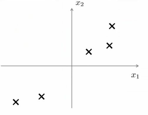
- In other words, find a single line onto which to project this data
  - How do we determine this line?
    - The distance between each point and the projected version should be small (blue lines below are short)
    - PCA tries to find a lower dimensional surface so the sum of squares onto that surface is minimized
    - The blue lines are sometimes called the projection error
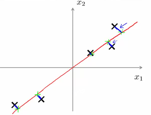
      - PCA tries to find the surface (a straight line in this case) which has the minimum projection error
    - As an aside, you should normally do mean normalization and feature scaling on your data before PCA
A more formal description is
- For 2D-1D, we must find a vector u⁽¹⁾, which is of some dimensionality
- Onto which you can project the data so as to minimize the projection error
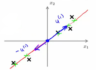
- u⁽¹⁾ can be positive or negative (-u⁽¹⁾) which makes no difference
  - Each of the vectors define the same red line
In the more general case
- To reduce from nD to kD we
  - Find k vectors (u⁽¹⁾, u⁽²⁾, ... u^(k)) onto which to project the data to minimize the projection error
  - So lots of vectors onto which we project the data
  - Find a set of vectors which we project the data onto the linear subspace spanned by that set of vectors
    - We can define a point in a plane with k vectors
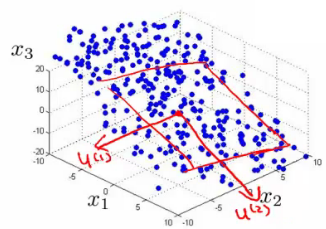
- e.g. 3D->2D
  - Find pair of vectors which define a 2D plane (surface) onto which you're going to project your data
  - Much like the "shallow box" example in compression, we're trying to create the shallowest box possible (by defining two of it's three dimensions, so the box's depth is minimized)
How does PCA relate to linear regression?
- PCA is not linear regression
  - Despite cosmetic similarities, very different
- For linear regression, fitting a straight line to minimize the squared distance between a point and the line
  - NB - VERTICAL distance between point
- For PCA minimizing the magnitude of the shortest orthogonal distance
  - Gives very different effects
- More generally
  - With linear regression we're trying to predict "y"
  - With PCA there is no "y" - instead we have a list of features and all features are treated equally
    - If we have 3D dimensional data 3D->2D
      - Have 3 features treated symmetrically

PCA Algorithm

Before applying PCA must do data preprocessing
- Given a set of m unlabeled examples we must do
  - Mean normalization
    - Replace each x_jⁱ with x_j - μ_j,
      - In other words, determine the mean of each feature set, and then for each feature subtract the mean from the value, so we re-scale the mean to be 0
  - Feature scaling (depending on data)
    - If features have very different scales then scale so they all have a comparable range of values
      - e.g. x_jⁱ is set to (x_j - μ_j) / s_j
        
        Where s_jis some measure of the range, so could be
        
        Biggest - smallest
        
        Standard deviation (more commonly)
With preprocessing done, PCA finds the lower dimensional sub-space which minimizes the sum of the squares
- In summary, for 2D->1D we'd be doing something like this;
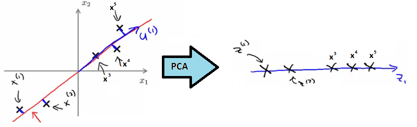
- Need to compute two things;
  - Compute the u vectors
    - The new planes
  - Need to compute the z vectors
    - z vectors are the new, lower dimensionality feature vectors
A mathematical derivation for the u vectors is very complicated
- But once you've done it, the procedure to find each u vector is not that hard

Algorithm description

Reducing data from n-dimensional to k-dimensional
- Compute the covariance matrix
  $Σ = \frac{1}{m} \sum_{i = 1}^{m} (x^{(i)}) {(x^{(i)})}^{T}$ The slide runs this sum to n, the number of features, where it has to run to m, the number of training examples — the 1/m in front of it is averaging over examples. Corrected here. Each term is an [n×1] column times a [1×n] row, so every one of them is [n×n], and so is Σ.
```
import numpy as np

rng = np.random.default_rng(0)
x1 = rng.normal(0, 1, 100)
X = np.c_[x1, 2 * x1 + rng.normal(0, 0.1, 100)]   # x2 is nearly 2*x1
X = X - X.mean(axis=0)                            # mean normalize first

Sigma = (X.T @ X) / len(X)          # the covariance matrix
U, S, Vt = np.linalg.svd(Sigma)
U[:, 0]   # [-0.446, -0.895] - the y = 2x direction (the sign is arbitrary),
          # i.e. [1, 2]/sqrt(5): the single direction the data really varies in
```
  PCA end to end on correlated data: the first column of U recovers the y = 2x line the data was generated along.
  - This is commonly denoted as Σ (greek upper case sigma) - NOT summation symbol
  - Σ = sigma
    - This is an [n x n] matrix
      - Remember that xⁱis a [n x 1] matrix
  - In Python we can implement this as follows;
```
Sigma = (X.T @ X) / m
```
    X holds the examples as rows, so X.T @ X sums the outer products in one matrix multiply — no loop over the m examples needed.
- Compute eigenvectors of matrix Σ
  - U, S, Vt = np.linalg.svd(Sigma)
    - svd = singular value decomposition
      - More numerically stable than np.linalg.eig
    - np.linalg.eig = also gives eigenvectors
- U,S and V are matrices
  - U matrix is also an [n x n] matrix
  - Turns out the columns of U are the u vectors we want!
  - So to reduce a system from n-dimensions to k-dimensions
    - Just take the first k-vectors from U (first k columns)
      
      $U = [\begin{matrix} | & | & | \\ u^{(1)} & u^{(2)} & \dots & u^{(n)} \\ | & | & | \end{matrix}] \in ℝ^{n \times n}$ One column per principal component, each a unit vector in the original n-dimensional space. Taking the first k columns gives U_reduce.
Next we need to find some way to change x (which is n dimensional) to z (which is k dimensional)
- (reduce the dimensionality)
- Take first k columns of the u matrix and stack in columns
  - n x k matrix - call this U_reduce
- We calculate z as follows
  - z = (U_reduce)^T * x
    - So [k x n] * [n x 1]
    - Generates a matrix which is
      - k * 1
    - If that's not witchcraft I don't know what is!
Exactly the same as with supervised learning except we're now doing it with unlabeled data
So in summary
- Preprocessing
- Calculate sigma (covariance matrix)
- Calculate eigenvectors with svd
- Take k vectors from U (U_reduce = U[:, :k])
- Calculate z (z = U_reduce.T @ x)
No mathematical derivation
- Very complicated
- But it works

Reconstruction from Compressed Representation

Earlier spoke about PCA as a compression algorithm
- If this is the case, is there a way to decompress the data from low dimensionality back to a higher dimensionality format?
Reconstruction
- Say we have an example as follows
  
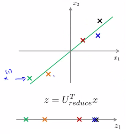  $z = U_{reduce}^{T} x$ U_reduce is [n×k], so its transpose times an [n×1] example gives the [k×1] vector z.
- We have our examples (x¹, x² etc.)
- Project onto z-surface
- Given a point z¹, how can we go back to the 2D space?
Considering
- z (vector) = (U_reduce)^T * x
To go in the opposite direction we must do
- x_approx = U_reduce * z
  - To consider dimensions (and prove this really works)
    - U_reduce = [n x k]
    - z [k * 1]
  - So
    - x_approx = [n x 1]
So this creates the following representation
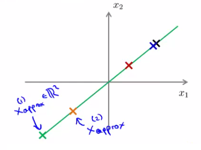
We lose some of the information (i.e. everything is now perfectly on that line) but it is now projected into 2D space

Choosing the number of Principal Components

How do we choose k ?
- k = number of principal components
- Guidelines about how to choose k for PCA
To choose k think about how PCA works
- PCA tries to minimize averaged squared projection error
  $\frac{1}{m} \sum_{i = 1}^{m} {‖ x^{(i)} - x_{approx}^{(i)} ‖}^{2}$
- Total variation in data can be defined as the average over data saying how far are the training examples from the origin
  $\frac{1}{m} \sum_{i = 1}^{m} {‖ x^{(i)} ‖}^{2}$
When we're choosing k typical to use something like this
$\frac{\frac{1}{m} \sum_{i = 1}^{m} {‖ x^{(i)} - x_{approx}^{(i)} ‖}^{2}}{\frac{1}{m} \sum_{i = 1}^{m} {‖ x^{(i)} ‖}^{2}} \leq 0.01 (1%)$ Projection error over total variation. At or below 0.01, 99% of the variance is retained.
```
k = 1
U_reduce = U[:, :k]              # keep one principal component
z = X @ U_reduce                 # project every example to 1-D
X_approx = z @ U_reduce.T        # reconstruct

num = ((X - X_approx) ** 2).sum(axis=1).mean()
den = (X ** 2).sum(axis=1).mean()
num / den   # 0.00039 -> 99.96% of the variance retained by one component
```
The variance-retained test on the data above: squashing 2-D to 1-D loses 0.04% of the variation, because the second dimension was almost entirely redundant.
- Ratio between averaged squared projection error with total variation in data
  - Want ratio to be small - means we retain 99% of the variance
- If it's small (0) then this is because the numerator is small
  - The numerator is small when xⁱ = x_approxⁱ
    - i.e. we lose very little information in the dimensionality reduction, so when we decompress we regenerate the same data
So we choose k in terms of this ratio
Often can significantly reduce data dimensionality while retaining the variance
How do you do this
$Algorithm:$ $Try PCA with k = 1$ $Compute U_{reduce}, z^{(1)}, z^{(2)}, \dots, z^{(m)}, x_{approx}^{(1)}, \dots, x_{approx}^{(m)}$ $Check if$ $\frac{\frac{1}{m} \sum_{i = 1}^{m} {‖ x^{(i)} - x_{approx}^{(i)} ‖}^{2}}{\frac{1}{m} \sum_{i = 1}^{m} {‖ x^{(i)} ‖}^{2}} \leq 0.01 ?$ If it fails, try k = 2, then k = 3, and so on. The chapter notes that the singular values from svd give the same answer far more cheaply, without recomputing PCA at every k.

Advice for Applying PCA

Can use PCA to speed up algorithm running time
- Explain how
- And give general advice

Speeding up supervised learning algorithms

Say you have a supervised learning problem
- Input x and y
  - x is a 10 000 dimensional feature vector
  - e.g. 100 x 100 images = 10 000 pixels
  - Such a huge feature vector will make the algorithm slow
- With PCA we can reduce the dimensionality and make it tractable
- How
  - 1) Extract xs
    - So we now have an unlabeled training set
  - 2) Apply PCA to x vectors
    - So we now have a reduced dimensional feature vector z
  - 3) This gives you a new training set
    - Each vector can be re-associated with the label
  - 4) Take the reduced dimensionality data set and feed to a learning algorithm
    - Use y as labels and z as feature vector
  - 5) If you have a new example map from higher dimensionality vector to lower dimensionality vector, then feed into learning algorithm
PCA maps one vector to a lower dimensionality vector
- x -> z
- Defined by PCA only on the training set
- The mapping computes a set of parameters
  - Feature scaling values
  - U_reduce
    - Parameter learned by PCA
    - Should be obtained only by determining PCA on your training set
- So we use those learned parameters for our
  - Cross validation data
  - Test set
Typically you can reduce data dimensionality by 5-10x without a major hit to algorithm

Applications of PCA

Compression
- Why
  - Reduce memory/disk needed to store data
  - Speed up learning algorithm
- How do we choose k?
  - % of variance retained
Visualization
- Typically choose k = 2 or k = 3
- Because we can plot these values!
One thing often done wrong regarding PCA
- A bad use of PCA: Use it to prevent over-fitting
  - Reasoning
    - If we have xⁱ we have n features, zⁱ has k features which can be lower
    - If we only have k features then maybe we're less likely to over fit...
  - This doesn't work
    - BAD APPLICATION
    - Might work OK, but not a good way to address over fitting
    - Better to use regularization
  - PCA throws away some data without knowing what values it's losing
    - Probably OK if you're keeping most of the data
    - But if you're throwing away some crucial data bad
    - So you have to go to like 95-99% variance retained
      - So here regularization will give you AT LEAST as good a way to solve over fitting
A second PCA myth
- Used for compression or visualization - good
- Sometimes used
  - Design ML system with PCA from the outset
    - But, what if you did the whole thing without PCA
  - See how a system performs without PCA
    - ONLY if you have a reason to believe PCA will help should you then add PCA
  - PCA is easy enough to add on as a processing step
    - Try without first!