02: Linear Regression with One Variable
What this chapter covers
- Chapter 01 was about what machine learning is - this is our first actual algorithm
- Linear regression with one variable - fit a straight line to some data
- Deliberately the simplest useful thing, because the point is the machinery around it
- Three pieces, and they show up again for essentially every algorithm in these notes
- Hypothesis - the function which does the predicting
- Cost function - a single number saying how wrong that function currently is
- Gradient descent - the procedure which changes the parameters to make that number smaller
- Worth getting comfortable here rather than rushing on
- This is the one problem simple enough to picture completely - two parameters, so the cost function is a surface you can actually look at
- That stops being true almost immediately afterwards
- But hypothesis -> cost -> minimize is exactly the pattern used for logistic regression, neural networks and everything after
Linear Regression
- Housing price data example used earlier
- Supervised learning regression problem
- What do we start with?
- Training set (this is your data set)
- Notation (used throughout the course)
- m = number of training examples
- x's = input variables / features
- y's = output variable "target" variables
- (x,y) - single training example
- (xi, yi) - specific example (ith training example)
- i is an index to training set
| Size in feet2 (x) | Price ($) in 1000's (y) |
|---|---|
| 2104 | 460 |
| 1416 | 232 |
| 1534 | 315 |
| 852 | 178 |
| … | … |
- With our training set defined - how do we used it?
- Take training set
- Pass into a learning algorithm
- Algorithm outputs a function (denoted h ) (h = hypothesis)
- This function takes an input (e.g. size of new house)
- Tries to output the estimated value of Y
- How do we represent hypothesis h ?
- Going to present h as;
- hθ(x) = θ0 + θ1x
- h(x) (shorthand)
- hθ(x) = θ0 + θ1x
- Going to present h as;
- What does this mean?
- Means Y is a linear function of x!
- θi are parameters
- θ0 is zero condition
- θ1 is gradient
- This kind of function is a linear regression with one variable
- Also called univariate linear regression
- So in summary
- A hypothesis takes in some variable
- Uses parameters determined by a learning system
- Outputs a prediction based on that input
Linear regression - implementation (cost function)
- A cost function lets us figure out how to fit the best straight line to our data
- Choosing values for θi (parameters)
- Different values give you different functions
- If θ0 is 1.5 and θ1 is 0 then we get straight line parallel with X along 1.5 @ y
- If θ1 is > 0 then we get a positive slope
- Based on our training set we want to generate parameters which make the straight line
- Chosen these parameters so hθ(x) is close to y for our training examples
- Basically, uses xs in training set with hθ(x) to give output which is as close to the actual y value as possible
- Think of hθ(x) as a "y imitator" - it tries to convert the x into y, and considering we already have y we can evaluate how well hθ(x) does this
- Chosen these parameters so hθ(x) is close to y for our training examples
- To formalize this;
- We want to solve a minimization problem
- Minimize (hθ(x) - y)2
- i.e. minimize the difference between h(x) and y for each/any/every example
- Sum this over the training set
- Minimize squared difference between predicted house price and actual house price
- 1/2m
- 1/m - means we determine the average
- 1/2m the 2 makes the math a bit easier, and doesn't change the constants we determine at all (i.e. half the smallest value is still the smallest value!)
- Minimizing θ0/θ1 means we get the values of θ0 and θ1 which find on average the minimal deviation of x from y when we use those parameters in our hypothesis function
- 1/2m
- More cleanly, this is a cost function
- And we want to minimize this cost function
- Our cost function is (because of the summation term) inherently looking at ALL the data in the training set at any time
- So to recap
- Hypothesis - is like your prediction machine, throw in an x value, get a putative y value
- Cost - is a way to, using your training data, determine values for your θ values which make the hypothesis as accurate as possible
J(θ0,θ1) is the cost function.
- This cost function is also called the squared error cost function
- This cost function is reasonable choice for most regression functions
- Probably most commonly used function
- This cost function is also called the squared error cost function
- In case J(θ0,θ1) is a bit abstract, going into what it does, why it works and how we use it in the coming sections
- Hypothesis - is like your prediction machine, throw in an x value, get a putative y value
Cost function - a deeper look
- Lets consider some intuition about the cost function and why we want to use it
- The cost function determines parameters
- The value associated with the parameters determines how your hypothesis behaves, with different values generate different
- Simplified hypothesis
- Assumes θ0 = 0
import numpy as np

x = np.array([1, 2, 3])   # the simplified data set used above
y = np.array([1, 2, 3])
m = 3

def J(theta1):            # cost with theta0 = 0
    return ((theta1 * x - y) ** 2).sum() / (2 * m)

J(1)      # 0.0    - a perfect fit
J(0.5)    # 0.583  - the ~0.58 read off the plot above
J(0)      # 2.333  - the ~2.3 read off the plot above
The three worked values from the bullets above, computed rather than read off the plot.
- Cost function and goal here are very similar to when we have θ0, but with a simpler parameter
- Simplified hypothesis makes visualizing cost function J() a bit easier
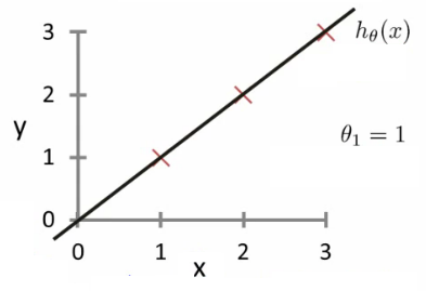
- So hypothesis passes through 0,0
- Two key functions we want to understand
- hθ(x)
- Hypothesis is a function of x - function of what the size of the house is
- J(θ1)
- Is a function of the parameter of θ1
- So for example
- θ1 = 1
- J(θ1) = 0
- Plot
- θ1 vs J(θ1)
- Data
- 1)
- θ1 = 1
- J(θ1) = 0
- 2)
- θ1 = 0.5
- J(θ1) = ~0.58
- 3)
- θ1 = 0
- J(θ1) = ~2.3
- 1)
- hθ(x)
- If we compute a range of values plot
- J(θ1) vs θ1 we get a polynomial (looks like a quadratic)
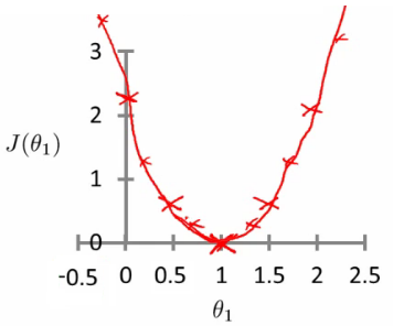
- J(θ1) vs θ1 we get a polynomial (looks like a quadratic)
- The optimization objective for the learning algorithm is find the value of θ1 which minimizes J(θ1)
- So, here θ1 = 1 is the best value for θ1
A deeper insight into the cost function - simplified cost function
- Assume you're familiar with contour plots or contour figures
- Using same cost function, hypothesis and goal as previously
- It's OK to skip parts of this section if you don't understand contour plots
- Using our original complex hypothesis with two variables,
- So cost function is
- J(θ0, θ1)
- So cost function is
- Example,
- Say
- θ0 = 50
- θ1 = 0.06
- Previously we plotted our cost function by plotting
- θ1 vs J(θ1)
- Now we have two parameters
- Plot becomes a bit more complicated
- Generates a 3D surface plot where axis are
- X = θ1
- Z = θ0
- Y = J(θ0,θ1)
- Say
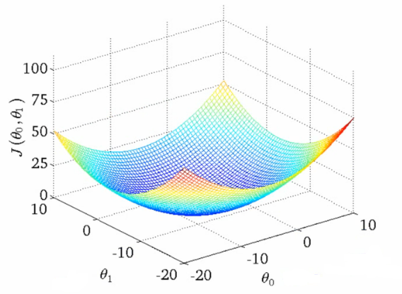
- We can see that the height (y) indicates the value of the cost function, so find where y is at a minimum
- Instead of a surface plot we can use a contour figures/plots
- Set of ellipses in different colors
- Each colour is the same value of J(θ0, θ1), but obviously plot to different locations because θ1 and θ0 will vary
- Imagine a bowl shape function coming out of the screen so the middle is the concentric circles
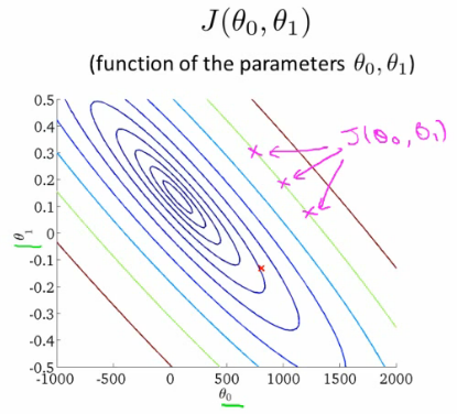
- Each point (like the red one above) represents a pair of parameter values for θ0 and θ1
- Our example here put the values at
- θ0 = ~800
- θ1 = ~-0.15
- Not a good fit
- i.e. these parameters give a value on our contour plot far from the center
- If we have
- θ0 = ~360
- θ1 = 0
- This gives a better hypothesis, but still not great - not in the center of the contour plot
- Finally we find the minimum, which gives the best hypothesis
- Our example here put the values at
- Doing this by eye/hand is a pain in the ass
- What we really want is an efficient algorithm for finding the minimum for θ0 and θ1
Gradient descent algorithm
- Minimize cost function J
- Gradient descent
- Used all over machine learning for minimization
- Start by looking at a general J() function
- Problem
- We have J(θ0, θ1)
- We want to get min J(θ0, θ1)
- Gradient descent applies to more general functions
- J(θ0, θ1, θ2 .... θn)
- min J(θ0, θ1, θ2 .... θn)
How does it work?
- Start with initial guesses
- Start at 0,0 (or any other value)
- Keeping changing θ0 and θ1 a little bit to try and reduce J(θ0,θ1)
- Each time you change the parameters, you select the gradient which reduces J(θ0,θ1) the most possible
- Repeat
- Do so until you converge to a local minimum
- Has an interesting property
- Where you start can determine which minimum you end up
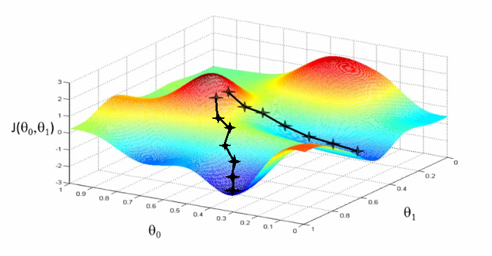
- Here we can see one initialization point led to one local minimum
- The other led to a different one
- Where you start can determine which minimum you end up
A more formal definition
- Do the following until convergence
for j = 0 and j = 1
- What does this all mean?
- Update θj by setting it to (θj - α) times the partial derivative of the cost function with respect to θj
- Notation
- :=
- Denotes assignment
- NB a = b is a truth assertion
- α (alpha)
- Is a number called the learning rate
- Controls how big a step you take
- If α is big have an aggressive gradient descent
- If α is small take tiny steps
- :=
- Derivative term
- Not going to talk about it now, derive it later
- There is a subtlety about how this gradient descent algorithm is implemented
- Do this for θ0 and θ1
- For j = 0 and j = 1 means we simultaneously update both
- How do we do this?
- Compute the right hand side for both θ0 and θ1
- So we need a temp value
- Then, update θ0 and θ1 at the same time
- We show this graphically below
- Compute the right hand side for both θ0 and θ1
Both parameters are updated from the old values — compute both temps first.
alpha = 0.1
h = theta0 + theta1 * x   # hypothesis for every example

temp0 = theta0 - alpha * (h - y).mean()
temp1 = theta1 - alpha * ((h - y) * x).mean()
theta0, theta1 = temp0, temp1   # update together, at the end
One simultaneous update, exactly as the equations above — both temps are computed from the old values before either parameter changes.
- If you implement the non-simultaneous update it's not gradient descent, and will behave weirdly
- But it might look sort of right - so it's important to remember this!
Understanding the algorithm
- To understand gradient descent, we'll return to a simpler function where we minimize one parameter to help explain the algorithm in more detail
- min θ1 J(θ1) where θ1 is a real number
- Two key terms in the algorithm
- Alpha
- Derivative term
- Notation nuances
- Partial derivative vs. derivative
- Use partial derivative when we have multiple variables but only derive with respect to one
- Use derivative when we are deriving with respect to all the variables
- Partial derivative vs. derivative
- Derivative term
- Derivative says
- Lets take the tangent at the point and look at the slope of the line
- So moving towards the minimum (down) will create a negative derivative, alpha is always positive, so will update J(θ1) to a smaller value
- Similarly, if the slope is positive the derivative term is positive, so θ1 is made smaller - again moving towards the minimum
- Derivative says
- Alpha term (α)
- What happens if alpha is too small or too large
- Too small
- Take baby steps
- Takes too long
- Too large
- Can overshoot the minimum and fail to converge
- When you get to a local minimum
- Gradient of tangent/derivative is 0
- So derivative term = 0
- alpha * 0 = 0
- So θ1 = θ1- 0
- So θ1 remains the same
- As you approach the global minimum the derivative term gets smaller, so your update gets smaller, even if alpha is fixed
- Means as the algorithm runs you take smaller steps as you approach the minimum
- So no need to change alpha over time
Linear regression with gradient descent
- Apply gradient descent to minimize the squared error cost function J(θ0, θ1)
- Now we have a partial derivative
- So here we're just expanding out the first expression
- J(θ0, θ1) = 1/2m....
- hθ(x) = θ0 + θ1*x
- So we need to determine the derivative for each parameter - i.e.
- When j = 0
- When j = 1
- Figure out what this partial derivative is for the θ0 and θ1 case
- When we derive this expression in terms of j = 0 and j = 1 we get the following
theta = np.zeros(2)
for _ in range(2000):
    h = theta[0] + theta[1] * x
    grad0 = (h - y).mean()           # the j = 0 derivative
    grad1 = ((h - y) * x).mean()     # the j = 1 derivative
    theta = theta - 0.1 * np.array([grad0, grad1])

theta   # [0., 1.]  -> h(x) = 0 + 1x, the perfect fit, found by descent
Batch gradient descent run to convergence on the simple data set: it lands on θ0 = 0, θ1 = 1 with cost zero.
- To check this you need to know multivariate calculus
- So we can plug these values back into the gradient descent algorithm
- How does it work
- Risk of meeting different local optimum
- The linear regression cost function is always a convex function - always has a single minimum
- Bowl shaped
- One global optima
- So gradient descent will always converge to global optima
- In action
- Initialize values to
- θ0 = 900
- θ1 = -0.1
- Initialize values to
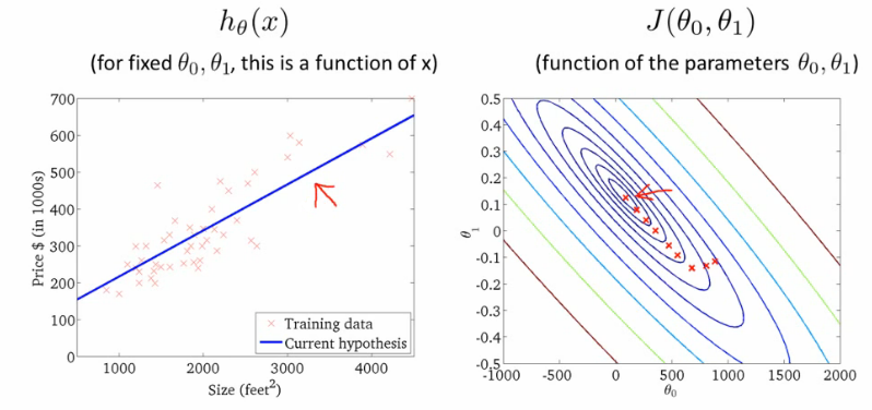
- End up at a global minimum
- This is actually Batch Gradient Descent
- Refers to the fact that over each step you look at all the training data
- Each step compute over m training examples
- Sometimes non-batch versions exist, which look at small data subsets
- We'll look at other forms of gradient descent (to use when m is too large) later in the course
- Refers to the fact that over each step you look at all the training data
- There exists an analytical solution for finding the minimum directly
- Normal equations method
- Gradient descent scales better to large data sets though
- Used in lots of contexts and machine learning
What's next - important extensions
Two extension to the algorithm
- 1) Normal equation for analytic solution
- To solve the minimization problem we can solve it [ min J(θ0, θ1) ] exactly using an analytic method which avoids the iterative approach used by gradient descent
- Normal equations method
- Has advantages and disadvantages
- Advantage
- No longer an alpha term
- Can be much faster for some problems
- Disadvantage
- Much more complicated
- Advantage
- We discuss the normal equation in the linear regression with multiple features section
- 2) We can learn with a larger number of features
- So may have other parameters which contribute towards a price
- e.g. with houses
- Size
- Age
- Number bedrooms
- Number floors
- x1, x2, x3, x4
- e.g. with houses
- With multiple features becomes hard to plot
- Can't really plot in more than 3 dimensions
- Notation becomes more complicated too
- Best way to get around this is the notation of linear algebra
- Gives notation and set of things you can do with matrices and vectors
- e.g. Matrix
- So may have other parameters which contribute towards a price
- We see here this matrix shows us
- Size
- Number of bedrooms
- Number floors
- Age of home
- All in one variable
- Block of numbers, take all data organized into one big block
- Vector
- Shown as y
- Shows us the prices
- Need linear algebra for more complex linear regression models
- Linear algebra is good for making computationally efficient models (as seen later too)
- Provide a good way to work with large sets of data sets
- Typically vectorization of a problem is a common optimization technique